enables you to make informed decisions about critical data in your enterprise.
Tip: You can find the PivotTable command on the Ribbon (Insert tab, Table group).
What is a Pivot Table?
A Pivot Table Report is an interactive way to quickly summarize large amounts of data. Use
a Pivot Table Report to analyse numerical data in detail and to answer unanticipated
questions about your data.

A Pivot Table Report is especially designed for:
– Querying large amounts of data in many user-friendly ways.
– Subtotaling and aggregating numeric data, summarizing data by categories and
subcategories, and creating custom calculations and formulas.
– Expanding and collapsing levels of data to focus your results, and drilling down to
details from the summary data for areas of interest to you.
– Moving rows to columns or columns to rows (or “pivoting”) to see different
summaries of the source data.
– Filtering, sorting, grouping, and conditionally formatting the most useful and
interesting subset of data to enable you to focus on the information that you want.
You often use a Pivot Table Report when you want to analyse related totals, especially when
you have a long list of figures to sum and you want to compare several facts about each
figure.
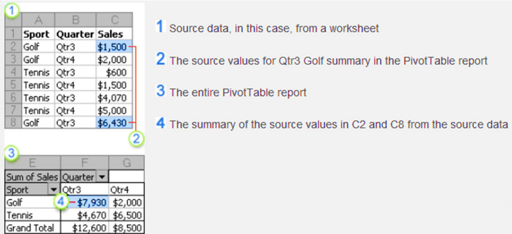
In the Pivot Table Report illustrated below, you can easily see how the third-quarter golf
sales in cell F3 compare to sales for another sport, or quarter, or to the total sales. In a Pivot Table Report, each column or field in your source data becomes a Pivot Table
Report field that summarizes multiple rows of information.
In the preceding example, the Sport column becomes the Sport field, and each record for Golf
is summarized in a single Golf item.
A value field, such as Sum of Sales, provides the values to be summarized. Cell F3 in the
preceding report contains the sum of the Sales value from every row in the source data for
which the Sport column contains Golf and the Quarter column contains Qtr3.
TIP: By default, data in the Values area summarize the underlying source data in the
PivotTable in the following way: numeric values use the SUM function, and text values use
the COUNT function.
To create a PivotTable report, you must define its source data, specify a location in the
workbook, and lay out the fields.
Ways to work with a PivotTable report
After you create the initial Pivot Table Report by defining the data source, arranging fields in
the Pivot Table field List, and choosing an initial layout, you can perform the following tasks
as you work with a Pivot Table Report:
– Explore the data by doing the following:
– Expand and collapse data, and show the underlying details that pertain to the
values.
– Sort, filter, and group fields and items.
– Change summary functions, and add custom calculations and formulas.
– Change the form layout and field arrangement by doing the following: Change the Pivot Table Report form: compact, outline, or tabular.
– Add, rearrange, and remove fields.
– Change the order of fields or items.
– Change the layout of columns, rows, and subtotals by doing the following:
– Turn column and row field headers on or off, or display or hide blank lines.
– Display subtotals above or below their rows.
– Adjust column widths on refresh.
– Move a column field to the row area or a row field to the column area.
– Merge or unmerge cells for outer row and column items.
– Change the display of blanks and errors by doing the following:
– Change how errors and empty cells are displayed.
– Change how items and labels without data are shown.
– Display or hide blank lines
– Change the format by doing the following:
– Manually and conditionally format cells and ranges.
– Change the overall PivotTable format style.
– Change the number format for fields.
Note: If you change the fields in the report after you’ve formatted them, either by
replacing them and/or adding/removing them, the formats will return to the
original format
Source Data:
You can use data from a Microsoft Excel worksheet as the basis for a report.
The data should be in list format, with column labels in the first row. Each cell in subsequent
rows should contain data appropriate to its column heading. There should not be any blank
rows or columns within the data of interest. Excel uses your column labels for the field names
in the report.
Using a Named Range: – To make the report easier to update, name the source range, and
use the name when you create the report. If the named range expands to include more data,
you can refresh the report to include the new data.
Excel Tables: – Excel tables are already in list format and are good candidates for PivotTable
source data. When you refresh the PivotTable report, new and updated data from the Excel
table is automatically included in the refresh operation.
Including Totals: – Excel automatically creates subtotals and grand totals in a PivotTable. If
The source data contains subtotals and grand totals that you created remove the subtotals and
grand totals before you create the report.