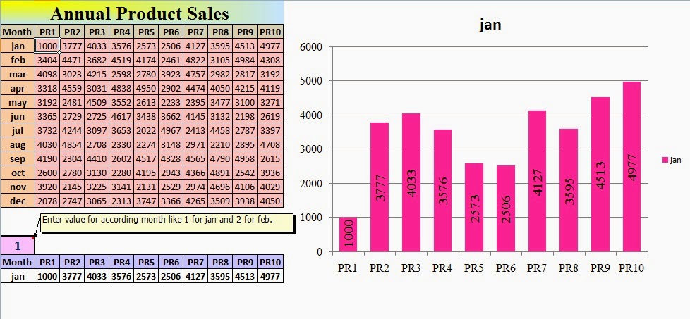
To create a chart, you must first enter the data for the chart on an Excel worksheet. Select that data, and then use the Chart Wizard to step through the process of selecting a chart type and the various chart options for your chart. To do this, follow these steps:
Start Excel, and then open your workbook.
Select the cells that contain the data that you want to display in your chart.
On the Insert menu, click Chart to start the Chart Wizard.
In the Chart Wizard – Step 1 of 4 – Chart Type dialog box, specify the chart type that you want to use for your chart. To do this, do one of the following:
Click the Standard Types tab. To view a sample of how your data will look when you select one of the standard chart types that Excel provides, click the chart type, click the chart subtype that you want to view, and then click Press and Hold to View Sample.
To select a chart type, click the chart type, click the chart subtype that you want, and then click Next.
Click the Custom Types tab. To select a built-in custom chart type, or to create your own chart type, click User-defined or Built-in. Select the chart type that you want, and then click Next.
In the Chart Wizard – Step 2 of 4 – Chart Source Data dialog box, you can specify the data range and how the series is displayed in your chart.

If the preview chart appears the way that you want, click Next.
If you want to change the data range or series for your chart, do any of the following, and then click Next.
On the Data Range tab, click the Data Range box, and then select the cells that you want on your worksheet.
Specify whether you want the series displayed in columns or rows.
On the Series tab, add and delete a series, or change the worksheet ranges used for the names and values for each series in your chart.
In the Chart Wizard – Step 3 of 4 – Chart Options dialog box, you can modify the appearance of your chart more when you select any of the chart option settings on the six tabs. As you change these settings, view the preview chart to make sure that your chart looks the way that you want.
When you finish selecting the chart options that you want, click Next.
On the Titles tab, you can add or change the chart and axis titles.
On the Axes tab, you can set the display options for the primary axes of your chart.
On the Gridlines tab, you can display or hide gridlines.
On the Legend tab, you can add a legend to your chart.
On the Data Labels tab, you can add data labels to your chart.
On the Data Table tab, you can display or hide data tables.
In the Chart Wizard – Step 4 of 4 – Chart Location dialog box, select the location in which to place your chart by doing one of the following:
Click As new sheet to display your chart as a new sheet.
Click As object in to display your chart as an object in a sheet.
Click Finish.
source:microsoft
CLICK HERE TO DOWNLOAD CREATABLE CHART EXCEL SHEET